Professional Trading Risk & Money Management

Before you begin

Risk and money management cannot make every trade win. It defines how much can be lost when an idea fails, how gains are harvested when it works, and whether the combined distribution remains compatible with capital and psychology. Every number below is educational; replace it with verified contract specifications, costs, and your own clean data.

Module 1: Foundation of Money Management

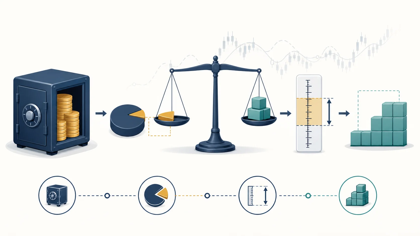
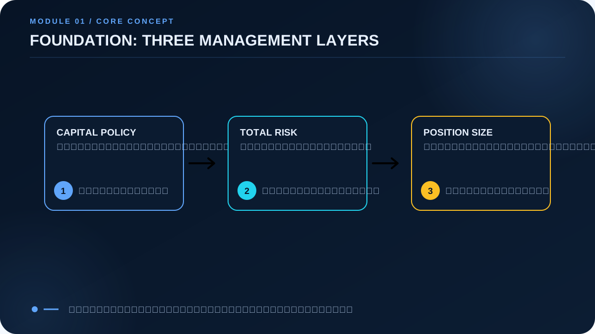
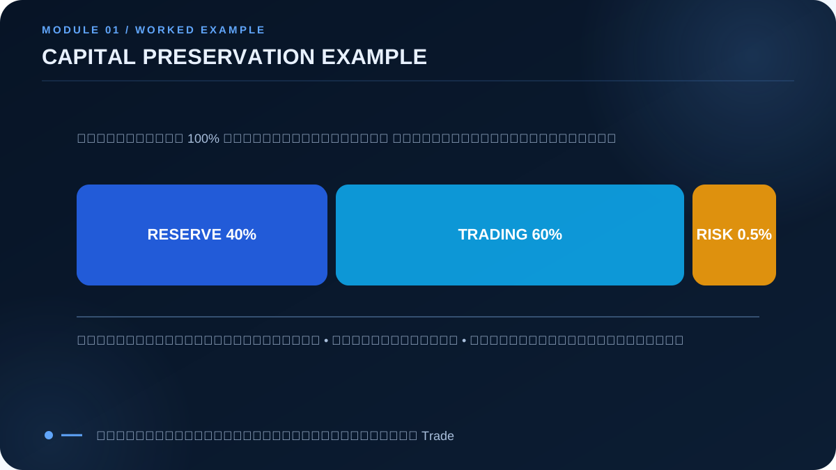
Money management sizes and allocates trading capital. Risk management also covers market, liquidity, operational, technology, concentration, and behavioral risk. Capital management governs reserves, withdrawals, deployment, and money that must never be exposed. Capital preservation means keeping the ability to continue, not avoiding every drawdown.

Trading edge is a repeatable positive statistical expectation after costs. It is not confidence. Entry, exit, market, time, size, and costs must be defined and tested over enough observations.

Module 2: Risk Metrics

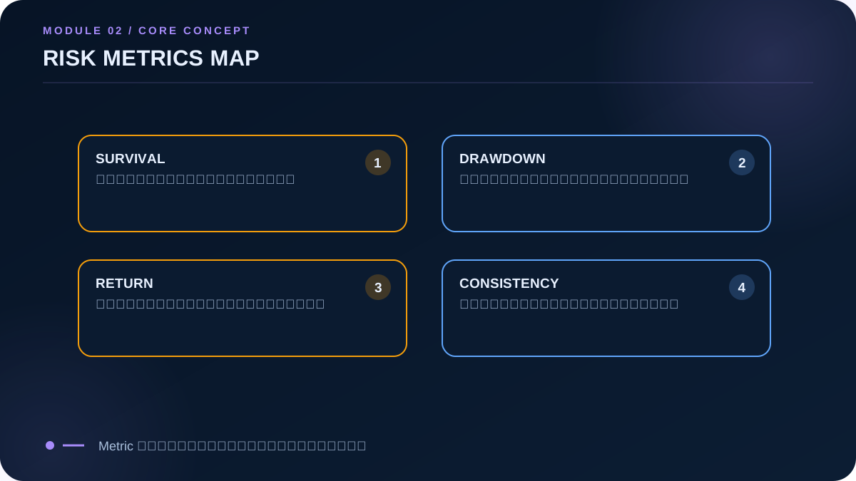
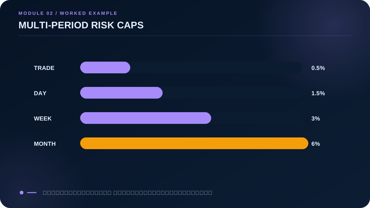
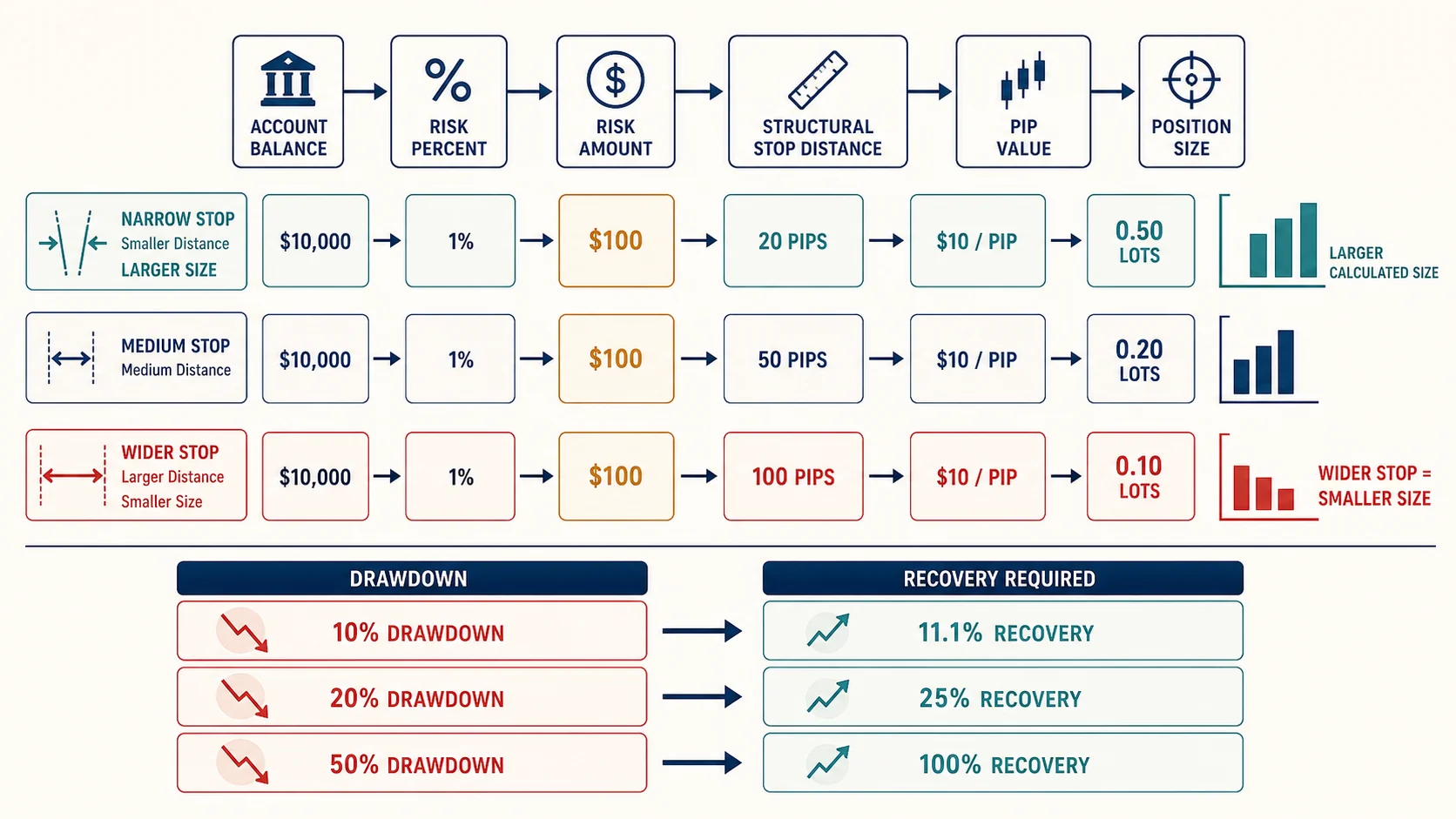
Set limits per trade, day, week, and month before trading. Maximum drawdown measures the largest peak-to-trough decline; specify balance or equity. Risk of ruin is model-dependent, not a certainty. Recovery Factor = Net Profit / Max Drawdown. Calmar commonly compares annual return with Max Drawdown. Basic Sharpe = excess mean return / return standard deviation, but it treats upside and downside variability alike.

Module 3: Position Sizing

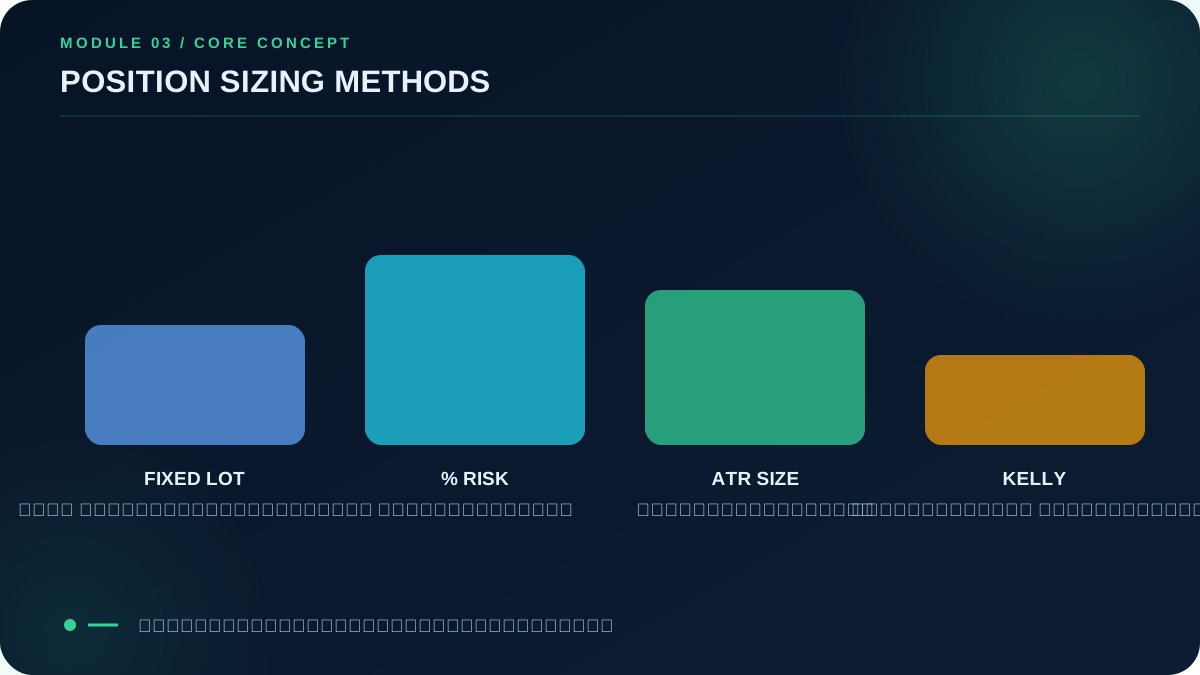
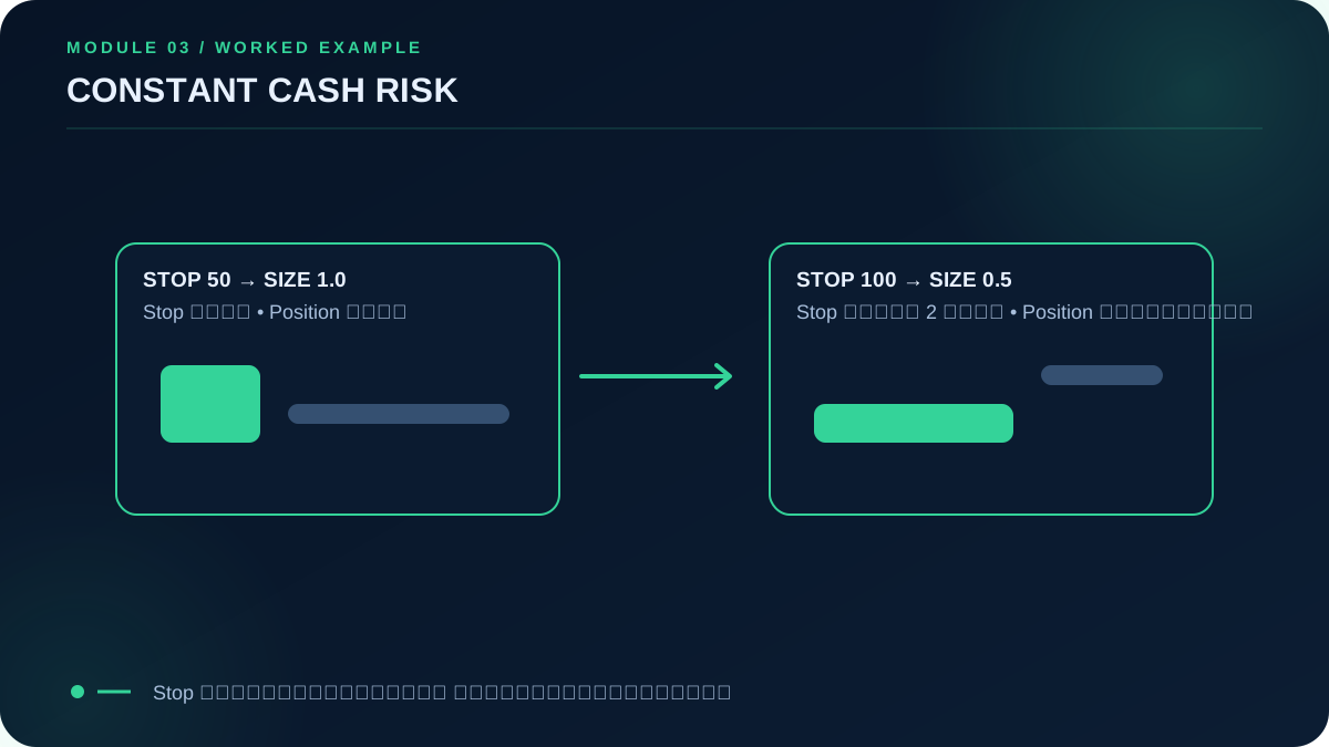
Fixed lot ignores changing stop distance and equity. Fixed fractional and percentage-risk sizing calculate size from current equity and invalidation distance. ATR and volatility sizing reduce size as movement expands. Kelly f* = p − q/b is highly sensitive to estimates; practical policies often use fractional Kelly plus a hard cap. Dynamic sizing must follow precommitted rules.

Module 4: Stop Loss Engineering

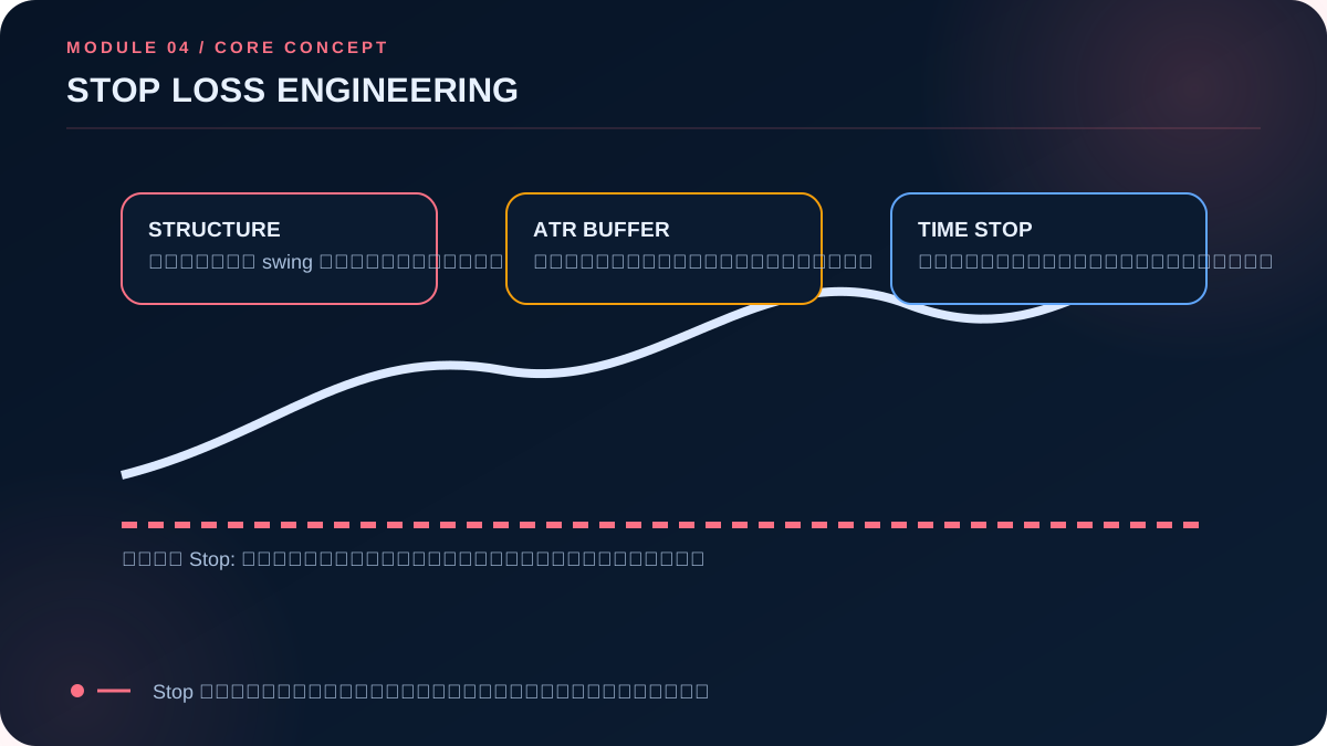
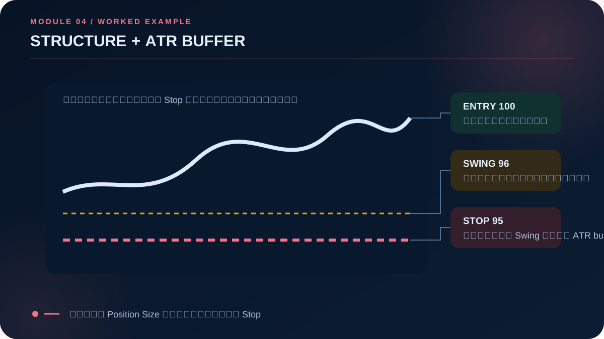
Technical and structure stops identify thesis failure. ATR and volatility stops normalize noise. Time stops exit when the expected development fails to occur. Initial stops define starting risk; trailing stops manage an already-developed position. Stops do not guarantee fills through gaps or thin liquidity.

Module 5: Reward Management

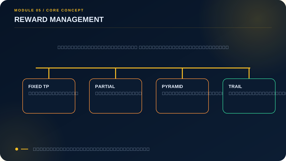
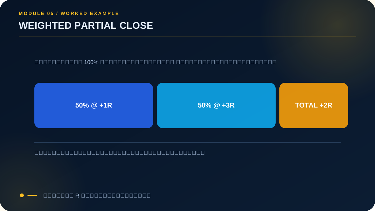
Risk–reward is incomplete without hit rate and costs. Partial closes, scaling out, pyramiding, and trailing exits reshape the outcome distribution. Predefine total risk and test identical rules across the sample.

Module 6: Trade Performance Analytics

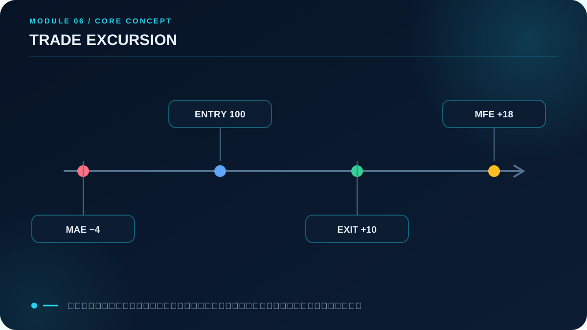
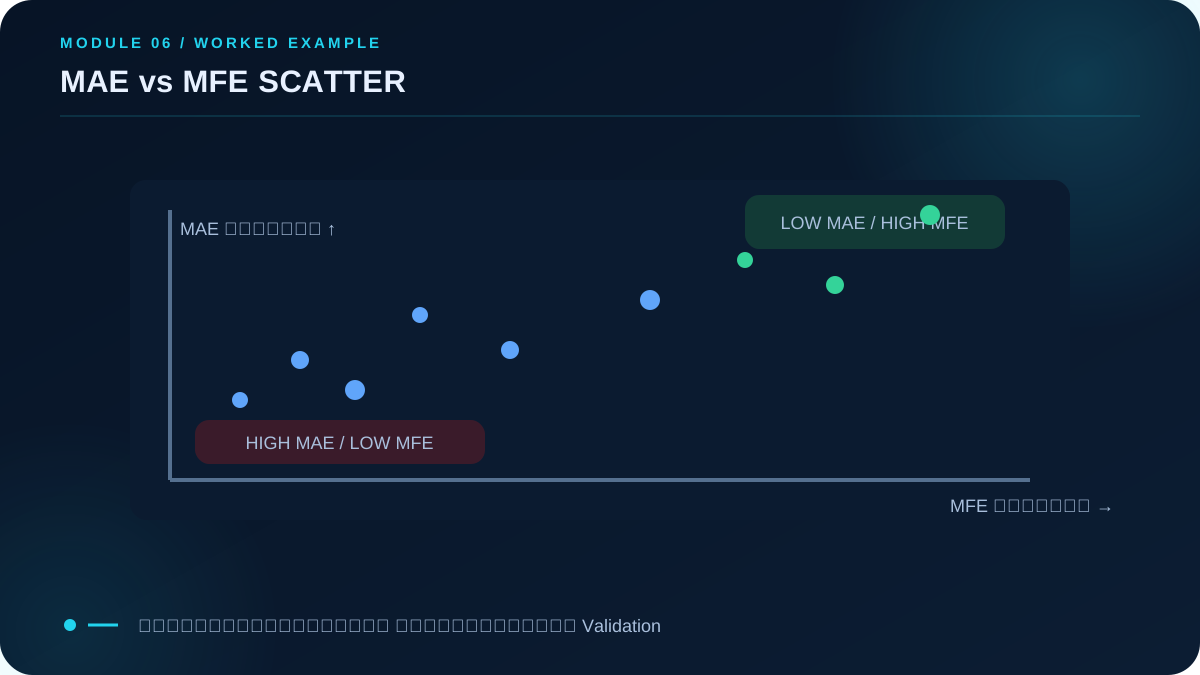
MAE (Maximum Adverse Excursion) is the worst adverse movement during a trade; MFE (Maximum Favorable Excursion) is the best favorable movement. Entry 100, low 96, high 118, exit 110 gives MAE −4, MFE +18, realized +10, and exit efficiency 10/18 = 55.6%. Standardize quote side and costs. Use MAE–MFE scatter plots on many trades, then validate any proposed stop or target on unseen data.

Module 7: R-Multiple and RPT

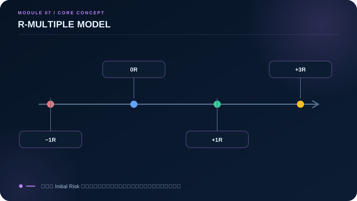
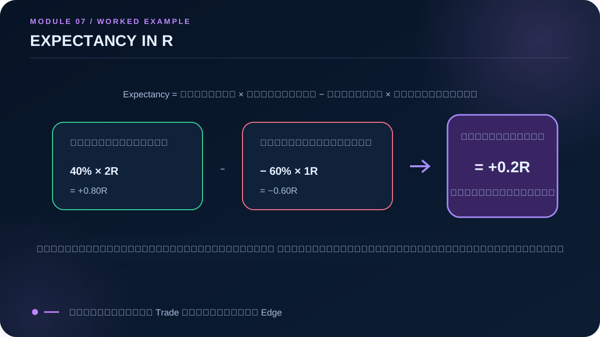
One R is initial planned risk. Expectancy in R = Win% × Avg Win R − Loss% × Avg Loss R. RPT may mean net profit per trade or average R per trade; state the unit. It enables comparison across different trade counts but does not show sequence risk or capital capacity.

Module 8: Equity Curve Analysis

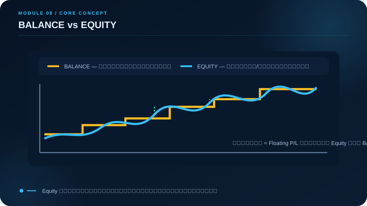
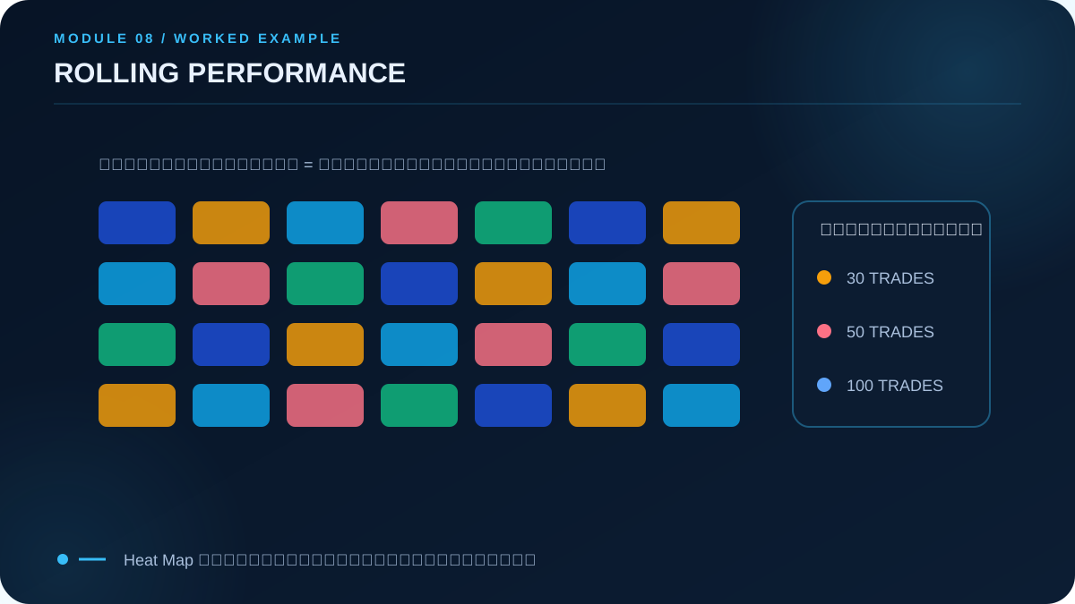
Balance changes on closed trades; equity includes open P/L. Track floating and closed drawdown, recovery, time under water, rolling performance, and heat maps with sample counts. A smooth curve can be misleading if open losses, future information, or overfitting are hidden.

Module 9: Portfolio Risk

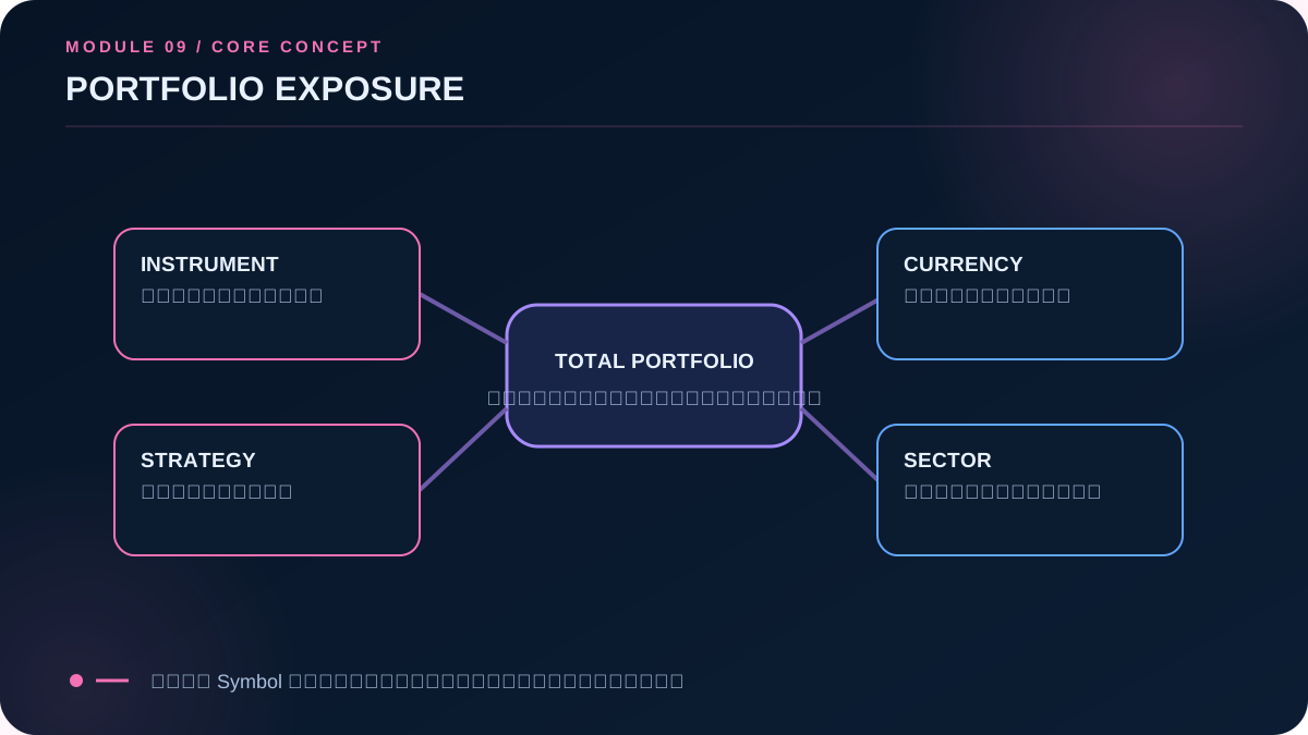
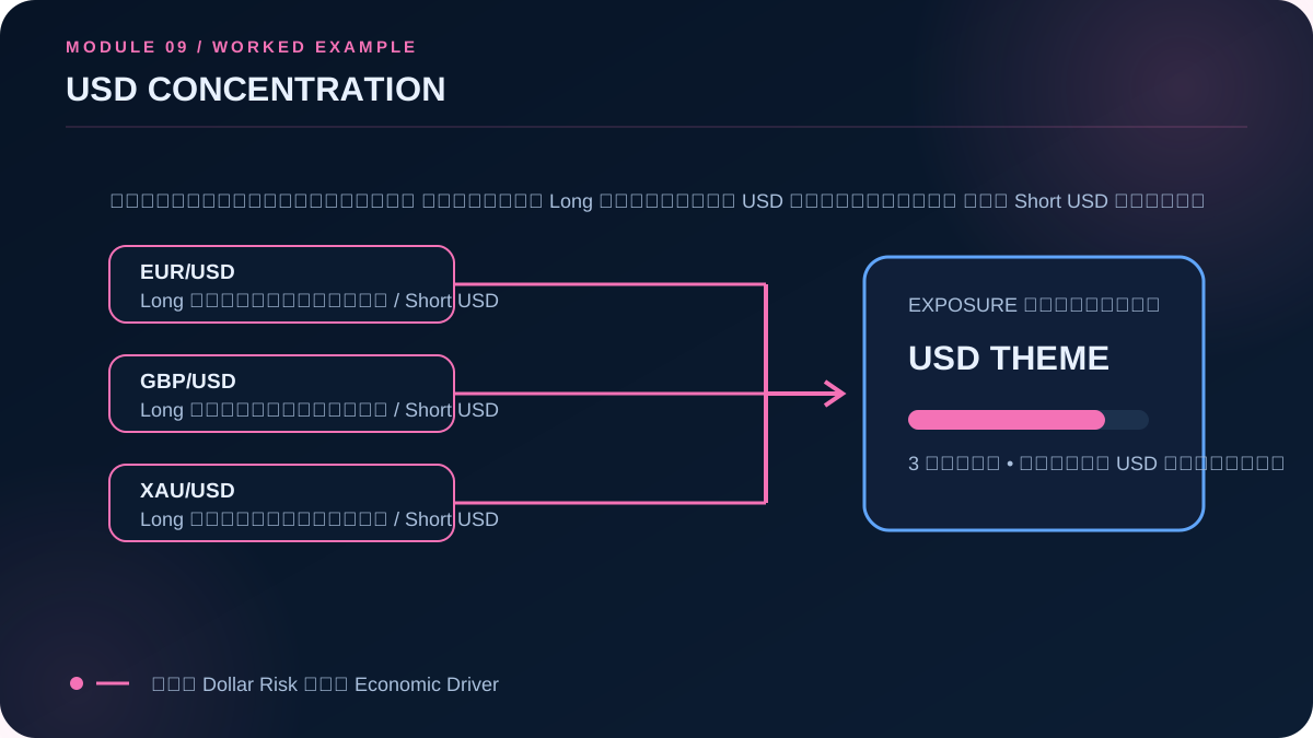
Measure correlation, dollar risk, strategy, sector, and currency exposure. EUR/USD long and GBP/USD long can both concentrate short-USD risk. Correlations change and often rise during stress, so use limits and scenarios rather than a short historical estimate alone.

Module 10: True Alpha Money Management

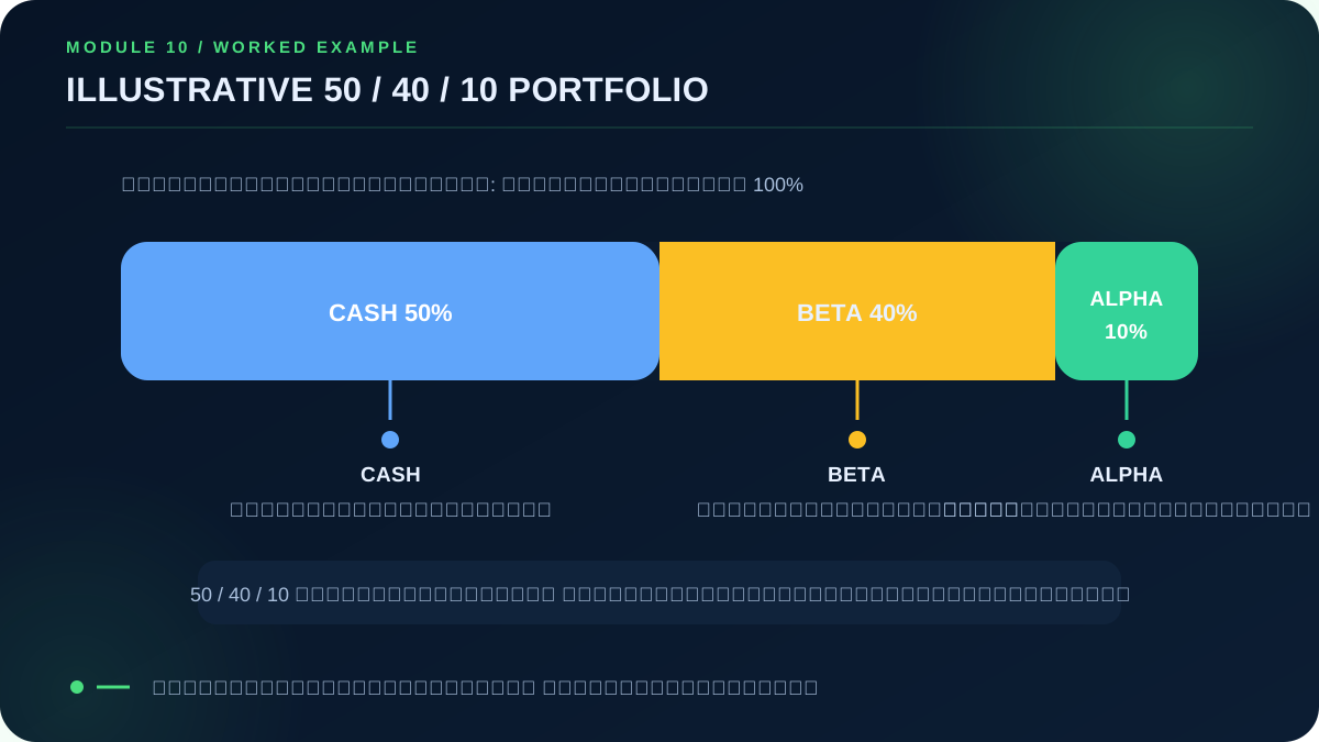
This lesson uses “True Alpha” as a portfolio-thinking framework, not a guaranteed-return claim or a universally standardized formula. Begin with the conceptual decomposition **Total return = Cash + Beta + Alpha**. Cash provides liquidity and resilience. Beta is return explained by systematic market exposure relative to an appropriate benchmark. Alpha is residual return above that benchmark after spreads, commissions, slippage, and other costs; it must be supported by adequate out-of-sample evidence.

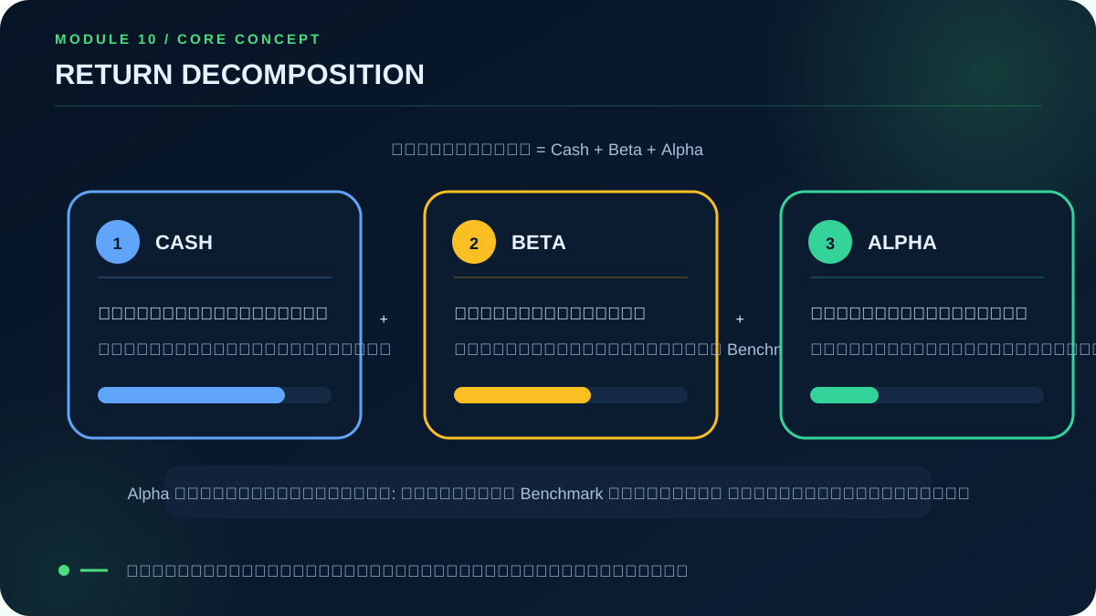
The supplied community article illustrates a 50% Cash, 40% Beta, and 10% Alpha portfolio. Treat those numbers as a teaching example, not a prescription. If the alpha sleeve lacks robust evidence, it should be reduced or omitted rather than expanded after a short winning period.

Return decomposition does not set risk limits. Add a separate risk overlay covering total portfolio risk, factor concentration, risk per trade, drawdown protection, and system suspension rules. Compound from current equity and scale only when rolling expectancy, profit factor, MAE/MFE, correlation, and sample size remain acceptable. Setup grades and escalation rules must be defined before outcomes are known.

Module 11: Monte Carlo and Robustness

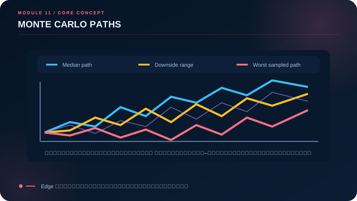
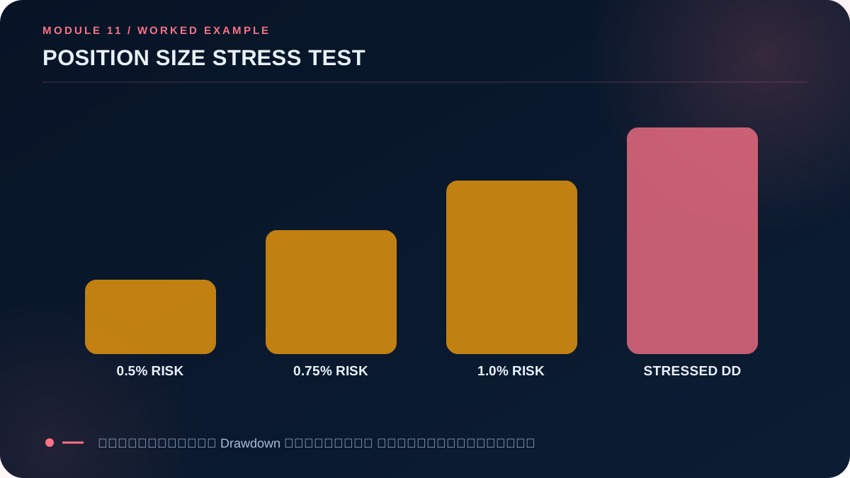
Monte Carlo resamples possible outcome sequences to estimate ranges of drawdown and ending equity. It does not create an edge. Confidence intervals inherit model assumptions; regime dependence and fat tails can make reality worse. Stress costs, correlation, edge decay, gaps, and position size.

Module 12: Trading Journal and Dashboard

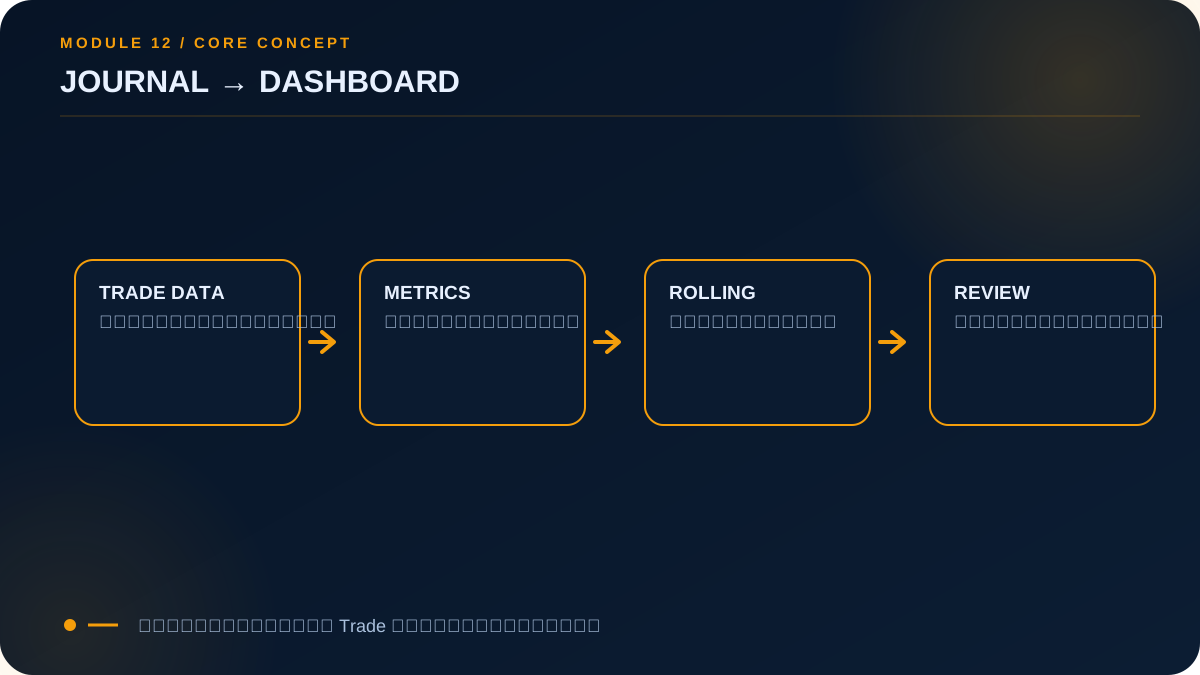
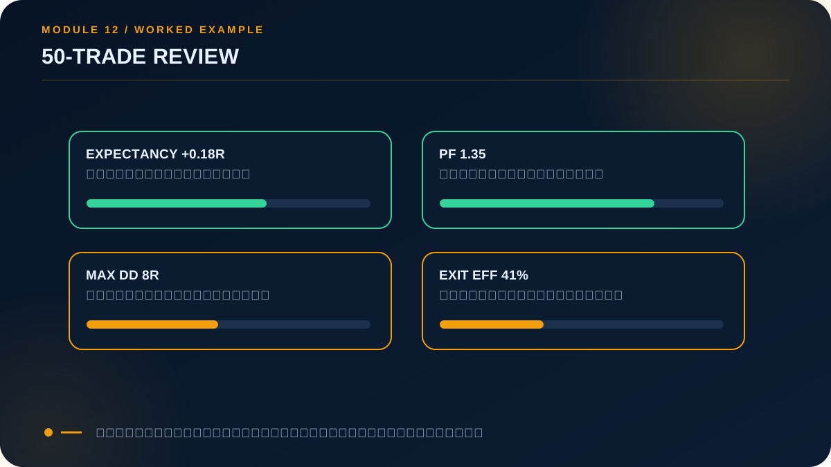
Capture timestamp, instrument, setup version, entry, stop, exit, initial risk, size, costs, slippage, MAE, MFE, R, screenshots, and exit reason. Lock pre-trade fields before the outcome. Track win rate, payoff, expectancy, profit factor, excursions, exit efficiency, RPT, drawdown, recovery, SQN (System Quality Number), equity, and rolling 30–100 trades. SQN = √N × Mean R / Standard Deviation R and must be reported with sample size and distribution.

Practical sequence

1. Document an after-cost edge.
2. Define thesis invalidation and worst-case loss.
3. Size from current equity and risk caps.
4. Check portfolio exposure and drawdown state.
5. Execute a checklist and lock pre-trade data.
6. Review MAE, MFE, R, expectancy, and equity in batches.
7. Stress test and adjust only through validated rules.